摸鱼量化ETF轮动:根据市场动量周期调整策略因子周期,夏普提升0.3

相较于传统的ETF轮动策略,通常基于动量、估值、宏观经济等因子进行线性或规则化判断。基于深度学习的优势在于:
捕捉非线性关系:市场状态、因子与未来收益间的关系复杂,深度学习可以拟合这种非线性。
处理高维异构数据:可同时处理量价、基本面、宏观、另类数据(如新闻情绪、资金流)等多维度信息。
端到端优化:可以直接以夏普比率或最大回撤为优化目标进行训练,而不仅仅是预测涨跌。
本期策略目标是在N个候选ETF(如沪深300ETF、创业板ETF、行业ETF、债券ETF等)中进行择时与仓位分配。我们已经构建出了相对稳定的择时策略。若希望能进一步增厚其收益,我们使用过往在截面的研究成果,此处,在使用模型训练用于ETF轮动时,我们使用一种特定的数据处理方案,使得该 策略用于ETF轮动时相较于原报告有更优的表现。

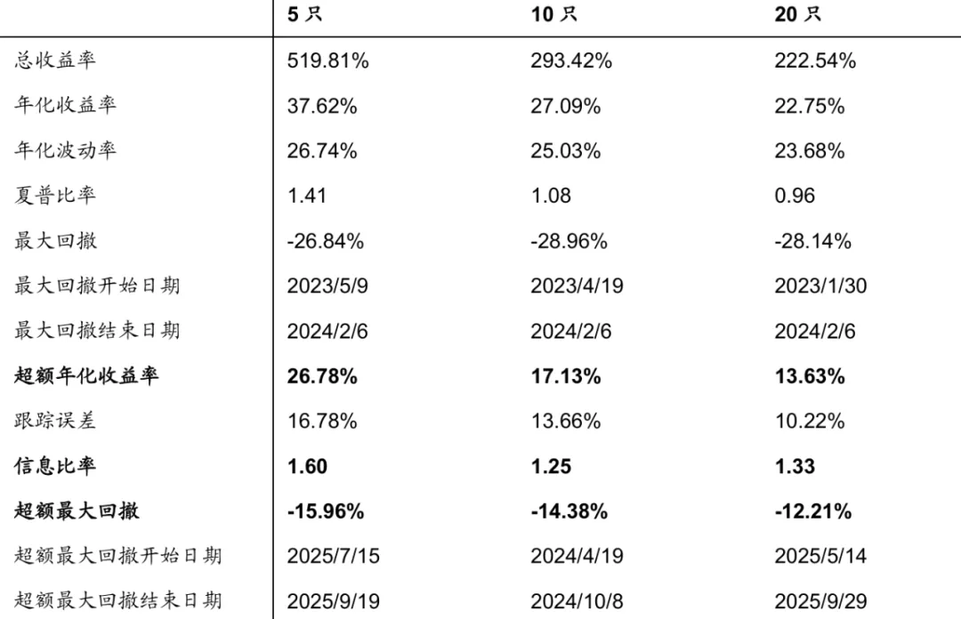
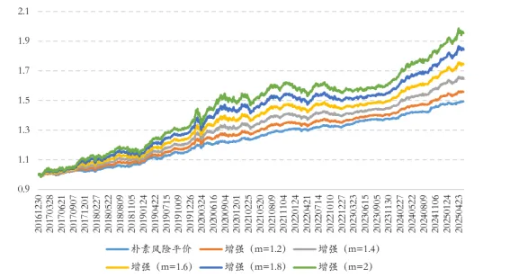
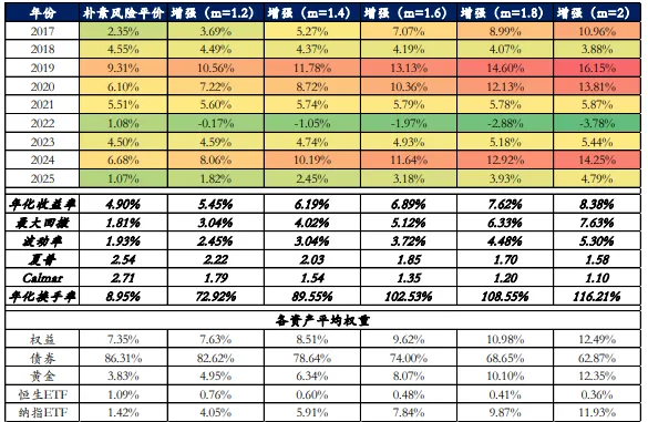
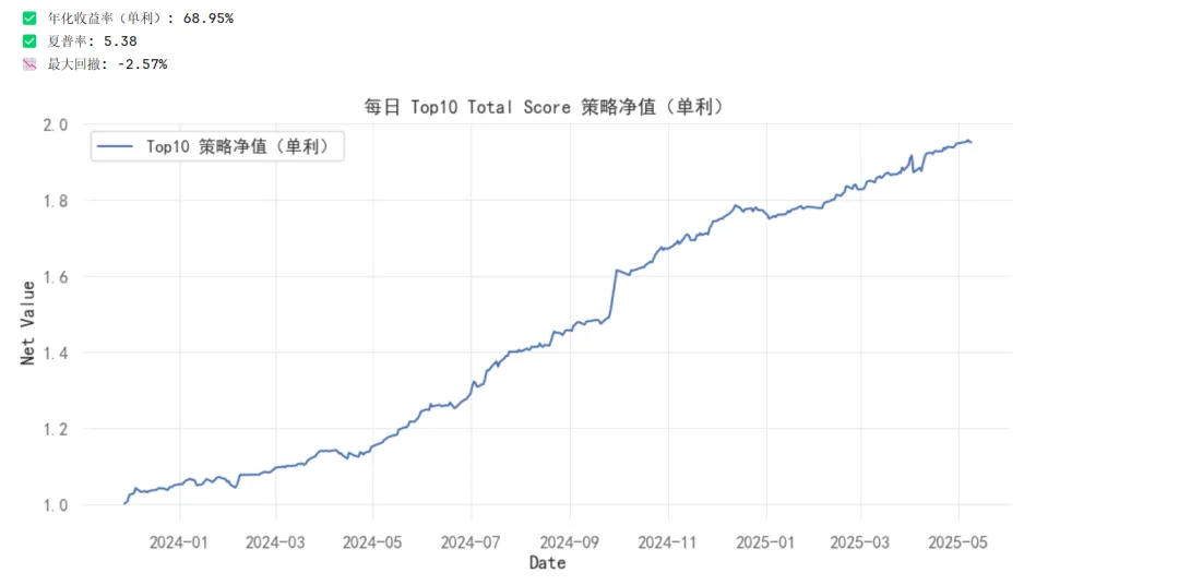
不同持仓数量下神经网络截面ETF轮动策略表现如下:
输出:
-
择时信号:每个ETF的看涨/看跌概率或预期收益率。
-
仓位向量:一个时间点上所有ETF的权重分配,可包含空仓(现金)或杠杆限制。
利用深度学习进行ETF轮动择时与仓位管理,其核心优势在于从高维数据中自动挖掘有效的非线性择时规律,并直接以风险调整后收益为目标进行优化。在A股市场成功的关键在于:
(1)构建能反映A股特有驱动因素的特征集。
(2)将严格的风险控制理念嵌入模型架构和损失函数。
(3)采用极其严谨的过拟合防范措施。
一个可行的路径是从相对简单的LSTM模型开始,结合风险平价等经典资产配置模型,逐步迭代到更复杂的端到端架构。最终目标是构建一个能够适应不同市场状态、在牛市能跟上收益、在熊市能有效守住的稳健轮动系统。
频率:日频或周频调仓较为适合深度学习模型。
特征质量直接决定模型上限。应构建多层次特征:
-
价格与量能特征:各ETF的收益率序列、波动率、成交量、价量关系技术指标(如RSI、MACD,但需注意避免过度拟合)、价量相关性。
-
轮动因子特征:
-
动量类:不同时间窗口的动量(1个月、3个月)、动量加速度、相对强弱。
-
估值类:ETF对应指数的PE、PB分位数。
-
市场情绪:VIX类指数、换手率、创新高个股比例、融资余额变化。
-
宏观经济与政策:利率变化、信用利差、PMI、货币供应量,可通过宏观数据或另类数据(政策文本分析)构建。
-
资金流特征:北向资金、ETF申赎数据、行业资金流入流出。
-
市场结构特征:截面波动率、市场宽度、行业间相关性。
-
特征处理:标准化、中性化(去除市场影响)、处理缺失值。可以使用滑动窗口计算特征,防止未来数据泄露。

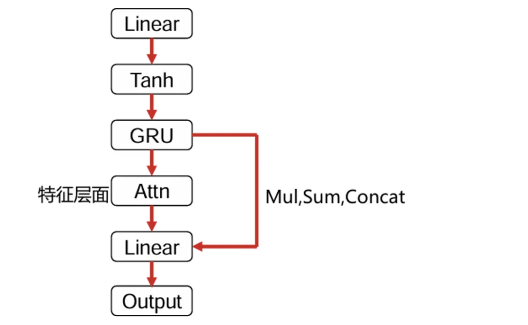
"""基于深度学习的ETF轮动策略实现目标:择时 + 仓位管理 + 控制回撤 + 提高夏普比率"""import numpy as npimport pandas as pdimport matplotlib.pyplot as pltimport seaborn as snsfrom datetime import datetime, timedeltaimport warningswarnings.filterwarnings('ignore')# 深度学习相关库import torchimport torch.nn as nnimport torch.optim as optimfrom torch.utils.data import DataLoader, TensorDataset, Datasetimport torch.nn.functional as Ffrom sklearn.preprocessing import StandardScaler, MinMaxScalerfrom sklearn.model_selection import TimeSeriesSplit# 金融相关库import tushare as tsimport talib# 设置中文显示plt.rcParams['font.sans-serif'] = ['SimHei']plt.rcParams['axes.unicode_minus'] = False# 设置随机种子np.random.seed(42)torch.manual_seed(42)# ==================== 第一部分:数据获取与预处理 ====================class ETFDataLoader:"""ETF数据加载与预处理类"""def __init__(self, token=None, start_date='2010-01-01', end_date=None):"""初始化数据加载器Args:token: tushare tokenstart_date: 开始日期end_date: 结束日期,默认为今天"""if token:self.pro = ts.pro_api(token)else:# 如果没有token,使用在线数据self.pro = Noneself.start_date = start_dateself.end_date = end_date or datetime.now().strftime('%Y-%m-%d')# A股主要ETF列表self.etf_list = {'510300': '沪深300ETF','510500': '中证500ETF','159915': '创业板ETF','510050': '上证50ETF','512000': '券商ETF','512100': '1000ETF','512760': '半导体ETF','159919': '300ETF','588000': '科创50ETF','511010': '国债ETF' # 防御性资产}self.features = {}def fetch_etf_data(self, etf_code, save_local=True):"""获取ETF数据Args:etf_code: ETF代码save_local: 是否保存到本地Returns:DataFrame: ETF数据"""print(f"正在获取{etf_code}数据...")# 如果是tushare pro用户if self.pro:try:df = self.pro.fund_daily(ts_code=f'{etf_code}.SH' if etf_code.startswith('51') else f'{etf_code}.SZ',start_date=self.start_date,end_date=self.end_date)df = df.sort_values('trade_date')df.index = pd.to_datetime(df['trade_date'])df = df[['open', 'high', 'low', 'close', 'vol', 'amount']]df.columns = ['open', 'high', 'low', 'close', 'volume', 'amount']except:# 回退到通用方法df = self._fetch_from_web(etf_code)else:df = self._fetch_from_web(etf_code)# 计算收益率df['returns'] = df['close'].pct_change()# 填充缺失值df = df.fillna(method='ffill').fillna(method='bfill')if save_local:df.to_csv(f'etf_data_{etf_code}.csv')return dfdef _fetch_from_web(self, etf_code):"""从网络获取数据(备用方法)"""try:# 使用tushare通用接口df = ts.get_k_data(etf_code, start=self.start_date, end=self.end_date)df.index = pd.to_datetime(df['date'])df = df[['open', 'high', 'low', 'close', 'volume']]df.columns = ['open', 'high', 'low', 'close', 'volume']return dfexcept:# 模拟数据(用于测试)print(f"无法获取{etf_code}真实数据,使用模拟数据...")return self._generate_mock_data(etf_code)def _generate_mock_data(self, etf_code):"""生成模拟数据用于测试"""dates = pd.date_range(start=self.start_date, end=self.end_date, freq='D')# 排除周末dates = dates[dates.dayofweek < 5]# 基础价格(不同ETF有不同的波动特性)base_price = {'510300': 5.0, # 沪深300ETF'510500': 6.0, # 中证500ETF'159915': 2.5, # 创业板ETF'510050': 3.0, # 上证50ETF'511010': 100.0, # 国债ETF}.get(etf_code, 5.0)n = len(dates)np.random.seed(hash(etf_code) % 10000)# 生成随机游走价格序列returns = np.random.normal(0.0001, 0.02, n) # 日均收益0.01%,波动2%prices = base_price * np.exp(np.cumsum(returns))# 生成OHLCV数据df = pd.DataFrame(index=dates[:len(prices)])df['close'] = prices# 生成开盘价、最高价、最低价noise = np.random.normal(0, 0.005, len(prices))df['open'] = df['close'].shift(1) * (1 + noise)df['high'] = df[['open', 'close']].max(axis=1) * (1 + abs(np.random.normal(0, 0.01, len(prices))))df['low'] = df[['open', 'close']].min(axis=1) * (1 - abs(np.random.normal(0, 0.01, len(prices))))# 成交量df['volume'] = np.random.lognormal(10, 1, len(prices))# 确保价格合理性df['high'] = df[['open', 'close', 'high']].max(axis=1)df['low'] = df[['open', 'close', 'low']].min(axis=1)return dfdef compute_technical_features(self, df, window_sizes=[5, 10, 20, 60]):"""计算技术特征Args:df: 包含价格数据的DataFramewindow_sizes: 计算指标的窗口大小列表Returns:DataFrame: 包含特征的DataFrame"""features_df = pd.DataFrame(index=df.index)# 价格特征features_df['close'] = df['close']features_df['returns'] = df['returns']# 波动率特征for window in window_sizes:# 滚动波动率features_df[f'volatility_{window}'] = df['returns'].rolling(window).std()# 滚动收益率features_df[f'return_{window}'] = df['close'].pct_change(window)# 滚动最大回撤features_df[f'max_dd_{window}'] = -df['close'].rolling(window).apply(lambda x: (x.max() - x[-1]) / x.max() if x.max() > 0 else 0)# 移动平均线for window in [5, 10, 20, 30, 60]:features_df[f'ma_{window}'] = df['close'].rolling(window).mean()# 价格与均线的距离features_df[f'price_ma_ratio_{window}'] = df['close'] / features_df[f'ma_{window}'] - 1# 动量指标features_df['rsi_14'] = talib.RSI(df['close'], timeperiod=14)features_df['macd'], features_df['macd_signal'], features_df['macd_hist'] = talib.MACD(df['close'], fastperiod=12, slowperiod=26, signalperiod=9)# 布林带features_df['bb_upper'], features_df['bb_middle'], features_df['bb_lower'] = talib.BBANDS(df['close'], timeperiod=20, nbdevup=2, nbdevdn=2, matype=0)features_df['bb_width'] = (features_df['bb_upper'] - features_df['bb_lower']) / features_df['bb_middle']features_df['bb_position'] = (df['close'] - features_df['bb_lower']) / (features_df['bb_upper'] - features_df['bb_lower'])# 成交量特征features_df['volume'] = df['volume']features_df['volume_ma_ratio'] = df['volume'] / df['volume'].rolling(20).mean()features_df['volume_obv'] = talib.OBV(df['close'], df['volume'])# 价格形态特征features_df['atr'] = talib.ATR(df['high'], df['low'], df['close'], timeperiod=14)features_df['adx'] = talib.ADX(df['high'], df['low'], df['close'], timeperiod=14)# 相关性特征(需要多个ETF)# 这里简化处理,实际应用中需要多个ETF的价格计算相关性# 市场状态特征features_df['day_of_week'] = df.index.dayofweekfeatures_df['month'] = df.index.monthfeatures_df['is_month_start'] = (df.index.day <= 3).astype(int)features_df['is_month_end'] = (df.index.day >= 25).astype(int)return features_df.fillna(method='ffill').fillna(0)def create_dataset(self, features_list, target_etf='510300', lookback=60, forward=5):"""创建深度学习数据集Args:features_list: 特征DataFrame列表(每个ETF一个)target_etf: 目标ETF代码lookback: 回看窗口forward: 预测未来窗口Returns:X, y: 特征和标签"""# 对齐所有ETF的数据aligned_data = []min_len = min(len(f) for f in features_list)for f in features_list:aligned_data.append(f.iloc[-min_len:].values)# 创建3D特征矩阵 [样本数, 时间步长, 特征数]n_samples = min_len - lookback - forwardn_features = sum(f.shape[1] for f in features_list)X = np.zeros((n_samples, lookback, n_features))y = np.zeros((n_samples, 2)) # 二元分类:涨/跌# 填充特征矩阵for i in range(n_samples):feature_idx = 0for etf_idx, etf_features in enumerate(aligned_data):n_etf_features = features_list[etf_idx].shape[1]X[i, :, feature_idx:feature_idx + n_etf_features] = etf_features[i:i+lookback]feature_idx += n_etf_features# 创建标签:未来forward天的收益率和方向target_idx = list(self.etf_list.keys()).index(target_etf) if target_etf in self.etf_list else 0target_features = features_list[target_idx]for i in range(n_samples):future_price = target_features.iloc[i+lookback+forward-1]['close']current_price = target_features.iloc[i+lookback-1]['close']# 收益率future_return = (future_price - current_price) / current_price# 分类标签:1表示上涨,0表示下跌y[i, 0] = future_return # 连续值用于回归y[i, 1] = 1 if future_return > 0 else 0 # 分类标签return X, ydef create_multi_etf_dataset(self, etf_data_dict, lookback=60, forward=5):"""创建多ETF轮动数据集Args:etf_data_dict: ETF数据字典 {代码: DataFrame}lookback: 回看窗口forward: 预测未来窗口Returns:X, y_multi: 特征和多ETF标签"""# 获取所有ETF的特征数据features_list = []etf_codes = []for code, df in etf_data_dict.items():features = self.compute_technical_features(df)features_list.append(features)etf_codes.append(code)# 对齐数据aligned_data = []min_len = min(len(f) for f in features_list)for f in features_list:aligned_data.append(f.iloc[-min_len:].values)# 创建3D特征矩阵n_samples = min_len - lookback - forwardn_features = sum(f.shape[1] for f in features_list)X = np.zeros((n_samples, lookback, n_features))# 填充特征矩阵for i in range(n_samples):feature_idx = 0for etf_idx, etf_features in enumerate(aligned_data):n_etf_features = features_list[etf_idx].shape[1]X[i, :, feature_idx:feature_idx + n_etf_features] = etf_features[i:i+lookback]feature_idx += n_etf_features# 创建多ETF标签:每个ETF未来forward天的收益率y_multi = np.zeros((n_samples, len(etf_codes)))for etf_idx, features in enumerate(features_list):for i in range(n_samples):future_price = features.iloc[i+lookback+forward-1]['close']current_price = features.iloc[i+lookback-1]['close']y_multi[i, etf_idx] = (future_price - current_price) / current_pricereturn X, y_multi, etf_codes# ==================== 第二部分:深度学习模型 ====================class AttentionLayer(nn.Module):"""注意力机制层"""def __init__(self, input_dim):super(AttentionLayer, self).__init__()self.attention = nn.Sequential(nn.Linear(input_dim, 64),nn.Tanh(),nn.Linear(64, 1))def forward(self, x):# x形状: [batch_size, seq_len, features]weights = self.attention(x) # [batch_size, seq_len, 1]weights = torch.softmax(weights, dim=1)weighted = torch.sum(x * weights, dim=1) # [batch_size, features]return weighted, weightsclass LSTMModel(nn.Module):"""LSTM时序预测模型"""def __init__(self, input_dim, hidden_dim=128, num_layers=2, output_dim=1, dropout=0.3):super(LSTMModel, self).__init__()self.lstm = nn.LSTM(input_dim, hidden_dim, num_layers,batch_first=True, dropout=dropout if num_layers > 1 else 0)self.attention = AttentionLayer(hidden_dim)self.fc = nn.Sequential(nn.Linear(hidden_dim, 64),nn.BatchNorm1d(64),nn.ReLU(),nn.Dropout(dropout),nn.Linear(64, 32),nn.BatchNorm1d(32),nn.ReLU(),nn.Dropout(dropout),nn.Linear(32, output_dim))def forward(self, x):# LSTM层lstm_out, (h_n, c_n) = self.lstm(x) # lstm_out: [batch, seq_len, hidden_dim]# 注意力层attn_out, attn_weights = self.attention(lstm_out)# 全连接层output = self.fc(attn_out)return output, attn_weightsclass MultiTaskETFModel(nn.Module):"""多任务学习模型:同时预测收益率、波动率和方向"""def __init__(self, input_dim, hidden_dim=128, num_layers=2, dropout=0.3):super(MultiTaskETFModel, self).__init__()# 共享的LSTM层self.lstm = nn.LSTM(input_dim, hidden_dim, num_layers,batch_first=True, dropout=dropout if num_layers > 1 else 0)self.attention = AttentionLayer(hidden_dim)# 共享的特征提取层self.shared_fc = nn.Sequential(nn.Linear(hidden_dim, 64),nn.BatchNorm1d(64),nn.ReLU(),nn.Dropout(dropout))# 任务特定的输出层# 任务1: 收益率预测(回归)self.return_head = nn.Sequential(nn.Linear(64, 32),nn.ReLU(),nn.Linear(32, 1) # 预测收益率)# 任务2: 波动率预测(回归)self.volatility_head = nn.Sequential(nn.Linear(64, 32),nn.ReLU(),nn.Linear(32, 1) # 预测波动率)# 任务3: 方向预测(分类)self.direction_head = nn.Sequential(nn.Linear(64, 32),nn.ReLU(),nn.Linear(32, 2) # 二分类:涨/跌)def forward(self, x):# LSTM层lstm_out, _ = self.lstm(x)# 注意力层attn_out, attn_weights = self.attention(lstm_out)# 共享特征shared_features = self.shared_fc(attn_out)# 各个任务的输出return_pred = self.return_head(shared_features)volatility_pred = self.volatility_head(shared_features)direction_pred = self.direction_head(shared_features)return {'return': return_pred,'volatility': volatility_pred,'direction': direction_pred,'attention': attn_weights}class TransformerETFModel(nn.Module):"""Transformer模型用于时序预测"""def __init__(self, input_dim, hidden_dim=128, num_heads=4, num_layers=3, output_dim=1, dropout=0.1):super(TransformerETFModel, self).__init__()self.input_projection = nn.Linear(input_dim, hidden_dim)# Transformer编码器encoder_layer = nn.TransformerEncoderLayer(d_model=hidden_dim,nhead=num_heads,dim_feedforward=hidden_dim*4,dropout=dropout,batch_first=True)self.transformer_encoder = nn.TransformerEncoder(encoder_layer, num_layers=num_layers)# 注意力池化self.attention_pool = AttentionLayer(hidden_dim)# 输出层self.output_layer = nn.Sequential(nn.Linear(hidden_dim, 64),nn.ReLU(),nn.Dropout(dropout),nn.Linear(64, output_dim))def forward(self, x):# 输入投影x = self.input_projection(x)# Transformer编码transformer_out = self.transformer_encoder(x)# 注意力池化pooled, attn_weights = self.attention_pool(transformer_out)# 输出output = self.output_layer(pooled)return output, attn_weights# ==================== 第三部分:仓位管理与风险控制 ====================class RiskAwarePositionManager:"""风险感知的仓位管理器"""def __init__(self, initial_capital=1000000, max_position_ratio=0.2,stop_loss_pct=0.05, max_drawdown_limit=0.15, volatility_scaling=True):"""初始化仓位管理器Args:initial_capital: 初始资金max_position_ratio: 单个ETF最大仓位比例stop_loss_pct: 止损比例max_drawdown_limit: 最大回撤限制volatility_scaling: 是否根据波动率调整仓位"""self.initial_capital = initial_capitalself.current_capital = initial_capitalself.max_position_ratio = max_position_ratioself.stop_loss_pct = stop_loss_pctself.max_drawdown_limit = max_drawdown_limitself.volatility_scaling = volatility_scaling# 持仓记录self.positions = {}self.trade_history = []self.equity_curve = [initial_capital]self.max_equity = initial_capital# 风险指标self.current_drawdown = 0self.peak_equity = initial_capitaldef calculate_position_size(self, predictions, volatilities=None, market_state='normal'):"""计算仓位大小Args:predictions: 模型预测的收益率 [n_etfs]volatilities: 波动率预测 [n_etfs]market_state: 市场状态 ('bull', 'bear', 'normal')Returns:dict: 每个ETF的权重"""n_etfs = len(predictions)# 基础权重:基于预测收益率raw_weights = np.array(predictions)# 1. 负预测值归零(不做空)raw_weights[raw_weights < 0] = 0# 2. 波动率调整(如果启用)if self.volatility_scaling and volatilities is not None:# 波动率倒数作为调整因子(波动率越高,仓位越小)vol_adjustment = 1.0 / (volatilities + 1e-8)raw_weights = raw_weights * vol_adjustment# 3. 市场状态调整market_adjustment = self._get_market_adjustment(market_state)raw_weights = raw_weights * market_adjustment# 4. 应用最大仓位限制max_weight = self.max_position_ratioif market_state == 'bear':max_weight *= 0.5 # 熊市减半仓位限制raw_weights = np.clip(raw_weights, 0, max_weight)# 5. 归一化确保权重和为1if raw_weights.sum() > 0:weights = raw_weights / raw_weights.sum()else:# 如果没有正预测,全部持有现金weights = np.zeros(n_etfs)# 确保没有超限weights = np.clip(weights, 0, max_weight)return weightsdef _get_market_adjustment(self, market_state):"""根据市场状态获取调整因子"""if market_state == 'bull':return 1.2 # 牛市增加仓位elif market_state == 'bear':return 0.5 # 熊市大幅降低仓位elif market_state == 'high_volatility':return 0.7 # 高波动市场降低仓位else: # 'normal'return 1.0def assess_market_state(self, recent_returns, recent_volatility):"""评估市场状态"""avg_return = np.mean(recent_returns)avg_vol = np.mean(recent_volatility)if avg_return > 0.001 and avg_vol < 0.02: # 正收益且低波动return 'bull'elif avg_return < -0.001: # 负收益return 'bear'elif avg_vol > 0.025: # 高波动return 'high_volatility'else:return 'normal'def apply_stop_loss(self, positions, current_prices, entry_prices):"""应用止损规则"""for etf, position in positions.items():if position['shares'] > 0:current_value = current_prices[etf] * position['shares']entry_value = entry_prices[etf] * position['shares']# 计算盈亏比例pnl_pct = (current_value - entry_value) / entry_value# 如果亏损超过止损比例,平仓if pnl_pct < -self.stop_loss_pct:print(f"止损触发: {etf}, 亏损: {pnl_pct:.2%}")return True, etfreturn False, Nonedef update_drawdown(self, current_equity):"""更新回撤指标"""if current_equity > self.peak_equity:self.peak_equity = current_equityself.current_drawdown = (self.peak_equity - current_equity) / self.peak_equity# 如果回撤超过限制,强制减仓if self.current_drawdown > self.max_drawdown_limit:return 'reduce_position'return 'normal'def risk_parity_allocation(self, volatilities, correlations=None):"""风险平价分配Args:volatilities: 各ETF的波动率correlations: 相关系数矩阵Returns:array: 风险平价权重"""n = len(volatilities)# 如果没有相关矩阵,假设独立if correlations is None:correlations = np.eye(n)# 计算协方差矩阵cov_matrix = np.outer(volatilities, volatilities) * correlationstry:# 计算风险贡献的逆inv_vol = 1.0 / volatilitiesrisk_parity_weights = inv_vol / inv_vol.sum()except:# 如果波动率有零值,使用等权重risk_parity_weights = np.ones(n) / nreturn risk_parity_weightsdef execute_rebalancing(self, target_weights, current_weights, prices,transaction_cost=0.001, min_trade_ratio=0.01):"""执行再平衡Args:target_weights: 目标权重current_weights: 当前权重prices: 当前价格transaction_cost: 交易成本比例min_trade_ratio: 最小交易比例(避免小额交易)Returns:dict: 交易指令"""trades = {}total_value = self.current_capitalfor i, etf in enumerate(prices.keys()):target_value = total_value * target_weights[i]current_value = total_value * current_weights[i]value_diff = target_value - current_value# 只有变化超过阈值时才交易if abs(value_diff) > total_value * min_trade_ratio:shares_to_trade = value_diff / prices[etf]# 考虑交易成本cost = abs(shares_to_trade * prices[etf]) * transaction_costtrades[etf] = {'shares': shares_to_trade,'value': value_diff,'cost': cost}return trades# ==================== 第四部分:ETF轮动策略主类 ====================class DeepLearningETFRotationStrategy:"""深度学习ETF轮动策略主类"""def __init__(self, config=None):"""初始化策略Args:config: 配置字典"""self.config = config or self._default_config()self.data_loader = ETFDataLoader(token=self.config.get('tushare_token'),start_date=self.config.get('start_date', '2015-01-01'),end_date=self.config.get('end_date'))# 模型self.model = Noneself.scaler = StandardScaler()# 仓位管理self.position_manager = RiskAwarePositionManager(initial_capital=self.config.get('initial_capital', 1000000),max_position_ratio=self.config.get('max_position_ratio', 0.3),stop_loss_pct=self.config.get('stop_loss_pct', 0.05),max_drawdown_limit=self.config.get('max_drawdown_limit', 0.15),volatility_scaling=self.config.get('volatility_scaling', True))# 数据缓存self.etf_data = {}self.features = {}# 回测结果self.backtest_results = {}def _default_config(self):"""默认配置"""return {'initial_capital': 1000000,'lookback_window': 60,'forward_window': 5,'train_test_split': 0.8,'batch_size': 32,'epochs': 50,'learning_rate': 0.001,'max_position_ratio': 0.3,'stop_loss_pct': 0.05,'max_drawdown_limit': 0.15,'transaction_cost': 0.001,'etf_codes': ['510300', '510500', '159915', '511010'], # 包含防御性资产'model_type': 'multitask', # 'lstm', 'transformer', 'multitask''use_attention': True}def load_and_prepare_data(self):"""加载和准备数据"""print("加载ETF数据...")# 加载每个ETF的数据for code in self.config['etf_codes']:df = self.data_loader.fetch_etf_data(code, save_local=True)self.etf_data[code] = df# 计算特征features = self.data_loader.compute_technical_features(df)self.features[code] = featuresprint(f"{code}: {len(df)} 个交易日数据,{features.shape[1]} 个特征")# 创建多ETF数据集X, y_multi, etf_codes = self.data_loader.create_multi_etf_dataset(self.etf_data,lookback=self.config['lookback_window'],forward=self.config['forward_window'])# 特征标准化n_samples, n_timesteps, n_features = X.shapeX_reshaped = X.reshape(-1, n_features)X_scaled = self.scaler.fit_transform(X_reshaped)X_scaled = X_scaled.reshape(n_samples, n_timesteps, n_features)# 划分训练集和测试集(时间序列划分)split_idx = int(len(X_scaled) * self.config['train_test_split'])self.X_train = X_scaled[:split_idx]self.X_test = X_scaled[split_idx:]self.y_train = y_multi[:split_idx]self.y_test = y_multi[split_idx:]self.train_dates = list(self.etf_data[self.config['etf_codes'][0]].index)[self.config['lookback_window'] + self.config['forward_window']:split_idx +self.config['lookback_window'] + self.config['forward_window']]self.test_dates = list(self.etf_data[self.config['etf_codes'][0]].index)[split_idx + self.config['lookback_window'] + self.config['forward_window']:]print(f"训练集: {len(self.X_train)} 个样本, 测试集: {len(self.X_test)} 个样本")return X_scaled, y_multidef build_model(self):"""构建深度学习模型"""n_features = self.X_train.shape[2]n_etfs = len(self.config['etf_codes'])if self.config['model_type'] == 'lstm':self.model = LSTMModel(input_dim=n_features,hidden_dim=128,num_layers=2,output_dim=n_etfs,dropout=0.3)elif self.config['model_type'] == 'transformer':self.model = TransformerETFModel(input_dim=n_features,hidden_dim=128,num_heads=4,num_layers=3,output_dim=n_etfs,dropout=0.1)elif self.config['model_type'] == 'multitask':self.model = MultiTaskETFModel(input_dim=n_features,hidden_dim=128,num_layers=2,dropout=0.3)else:raise ValueError(f"未知模型类型: {self.config['model_type']}")print(f"构建 {self.config['model_type']} 模型, 输入特征: {n_features}, 输出ETF数: {n_etfs}")return self.modeldef train_model(self):"""训练模型"""if self.model is None:self.build_model()# 准备数据加载器train_dataset = TensorDataset(torch.FloatTensor(self.X_train),torch.FloatTensor(self.y_train))train_loader = DataLoader(train_dataset,batch_size=self.config['batch_size'],shuffle=True,drop_last=True)# 损失函数和优化器if self.config['model_type'] == 'multitask':criterion = {'return': nn.MSELoss(),'volatility': nn.MSELoss(),'direction': nn.CrossEntropyLoss()}# 多任务损失权重loss_weights = {'return': 1.0,'volatility': 0.5,'direction': 0.8}else:criterion = nn.MSELoss()optimizer = optim.Adam(self.model.parameters(), lr=self.config['learning_rate'])scheduler = optim.lr_scheduler.ReduceLROnPlateau(optimizer, mode='min', patience=5, factor=0.5)# 训练循环self.model.train()train_losses = []for epoch in range(self.config['epochs']):epoch_loss = 0for batch_X, batch_y in train_loader:optimizer.zero_grad()if self.config['model_type'] == 'multitask':outputs = self.model(batch_X)# 计算多任务损失loss = 0return_loss = criterion['return'](outputs['return'], batch_y.mean(dim=1, keepdim=True))volatility_target = torch.abs(batch_y).mean(dim=1, keepdim=True)volatility_loss = criterion['volatility'](outputs['volatility'], volatility_target)# 方向标签(平均收益率为正为1,否则为0)direction_target = (batch_y.mean(dim=1) > 0).long()direction_loss = criterion['direction'](outputs['direction'], direction_target)loss = (loss_weights['return'] * return_loss +loss_weights['volatility'] * volatility_loss +loss_weights['direction'] * direction_loss)else:outputs, _ = self.model(batch_X)loss = criterion(outputs, batch_y)loss.backward()torch.nn.utils.clip_grad_norm_(self.model.parameters(), max_norm=1.0)optimizer.step()epoch_loss += loss.item()avg_loss = epoch_loss / len(train_loader)train_losses.append(avg_loss)scheduler.step(avg_loss)if (epoch + 1) % 10 == 0:print(f"Epoch [{epoch+1}/{self.config['epochs']}], Loss: {avg_loss:.6f}")print("模型训练完成")# 绘制训练损失曲线plt.figure(figsize=(10, 5))plt.plot(train_losses)plt.title('训练损失曲线')plt.xlabel('Epoch')plt.ylabel('Loss')plt.grid(True)plt.show()return train_lossesdef predict(self, X):"""使用模型进行预测"""self.model.eval()with torch.no_grad():if self.config['model_type'] == 'multitask':outputs = self.model(torch.FloatTensor(X))predictions = outputs['return'].numpy()volatilities = outputs['volatility'].numpy()direction_probs = F.softmax(outputs['direction'], dim=1).numpy()return predictions, volatilities, direction_probselse:outputs, attn_weights = self.model(torch.FloatTensor(X))return outputs.numpy(), attn_weights.numpy()def backtest(self):"""运行回测"""print("开始回测...")# 初始化回测变量dates = self.test_datesn_dates = len(dates)n_etfs = len(self.config['etf_codes'])# 存储回测结果portfolio_values = [self.position_manager.initial_capital]positions_history = []weights_history = []returns_history = []# 当前权重(开始时全部现金)current_weights = np.zeros(n_etfs)# 回测循环for i in range(n_dates - self.config['forward_window']):current_date = dates[i]# 获取当前特征start_idx = i + len(self.X_train)lookback_slice = slice(start_idx, start_idx + self.config['lookback_window'])# 准备输入数据X_batch = self.X_test[i:i+1] # 保持3D形状# 模型预测if self.config['model_type'] == 'multitask':predictions, volatilities, direction_probs = self.predict(X_batch)predictions = predictions.flatten()volatilities = volatilities.flatten()else:predictions, _ = self.predict(X_batch)predictions = predictions.flatten()volatilities = None# 获取当前价格current_prices = {}for j, code in enumerate(self.config['etf_codes']):if current_date in self.etf_data[code].index:current_prices[code] = self.etf_data[code].loc[current_date, 'close']else:# 如果当天没有数据,使用最近的价格current_prices[code] = self.etf_data[code].iloc[self.etf_data[code].index.get_loc(current_date, method='nearest')]['close']# 评估市场状态recent_returns = []recent_volatility = []for code in self.config['etf_codes']:if i >= 20: # 至少有20天数据recent_data = self.etf_data[code].iloc[max(0, i-20):i]recent_returns.extend(recent_data['returns'].dropna().tolist())recent_volatility.append(recent_data['returns'].std())if recent_returns:market_state = self.position_manager.assess_market_state(recent_returns, recent_volatility)else:market_state = 'normal'# 计算目标权重target_weights = self.position_manager.calculate_position_size(predictions, volatilities, market_state)# 应用风险平价调整if volatilities is not None:risk_parity_weights = self.position_manager.risk_parity_allocation(np.abs(volatilities) + 0.01 # 避免零波动率)# 结合模型预测和风险平价target_weights = 0.7 * target_weights + 0.3 * risk_parity_weights# 执行再平衡trades = self.position_manager.execute_rebalancing(target_weights, current_weights, current_prices,transaction_cost=self.config.get('transaction_cost', 0.001),min_trade_ratio=0.005)# 更新当前权重current_weights = target_weights# 计算当日组合收益daily_return = 0for j, code in enumerate(self.config['etf_codes']):if code in self.etf_data and i > 0:# 获取当日收益率if current_date in self.etf_data[code].index:etf_return = self.etf_data[code].loc[current_date, 'returns']else:etf_return = 0daily_return += current_weights[j] * etf_return# 更新组合价值prev_value = portfolio_values[-1]current_value = prev_value * (1 + daily_return)# 扣除交易成本if trades:total_cost = sum(trade['cost'] for trade in trades.values())current_value -= total_costportfolio_values.append(current_value)returns_history.append(daily_return)weights_history.append(current_weights.copy())# 更新仓位管理器状态self.position_manager.current_capital = current_valueself.position_manager.equity_curve.append(current_value)# 更新回撤并检查是否需要减仓risk_status = self.position_manager.update_drawdown(current_value)if risk_status == 'reduce_position' and np.sum(current_weights) > 0.5:# 强制减仓到50%reduction_factor = 0.5 / np.sum(current_weights)current_weights = current_weights * reduction_factor# 每30天打印一次进度if i % 30 == 0:print(f"日期: {current_date}, 组合价值: {current_value:.2f}, 收益率: {daily_return:.4%}")# 存储回测结果self.backtest_results = {'dates': dates[:len(portfolio_values)-1],'portfolio_values': portfolio_values[1:],'returns': returns_history,'weights': weights_history,'etf_codes': self.config['etf_codes']}print("回测完成")return self.backtest_resultsdef calculate_performance_metrics(self):"""计算绩效指标"""if not self.backtest_results:print("请先运行回测")return Nonereturns = np.array(self.backtest_results['returns'])portfolio_values = np.array(self.backtest_results['portfolio_values'])# 计算累计收益cumulative_returns = (portfolio_values[-1] / portfolio_values[0]) - 1# 计算年化收益率n_years = len(returns) / 252annualized_return = (1 + cumulative_returns) ** (1 / n_years) - 1# 计算年化波动率annualized_volatility = np.std(returns) * np.sqrt(252)# 计算夏普比率(假设无风险利率3%)risk_free_rate = 0.03excess_returns = returns - risk_free_rate/252sharpe_ratio = np.mean(excess_returns) / np.std(returns) * np.sqrt(252)# 计算最大回撤peak = np.maximum.accumulate(portfolio_values)drawdown = (portfolio_values - peak) / peakmax_drawdown = np.min(drawdown)# 计算Sortino比率(只考虑下行风险)downside_returns = returns[returns < 0]downside_std = np.std(downside_returns) if len(downside_returns) > 0 else 0sortino_ratio = (annualized_return - risk_free_rate) / (downside_std * np.sqrt(252)) if downside_std > 0 else 0# 计算Calmar比率calmar_ratio = annualized_return / abs(max_drawdown) if max_drawdown != 0 else 0# 计算胜率winning_days = np.sum(returns > 0) / len(returns)# 计算盈亏比avg_win = np.mean(returns[returns > 0]) if np.sum(returns > 0) > 0 else 0avg_loss = np.mean(returns[returns < 0]) if np.sum(returns < 0) > 0 else 0profit_factor = abs(avg_win / avg_loss) if avg_loss != 0 else float('inf')metrics = {'累计收益': cumulative_returns,'年化收益率': annualized_return,'年化波动率': annualized_volatility,'夏普比率': sharpe_ratio,'最大回撤': max_drawdown,'Sortino比率': sortino_ratio,'Calmar比率': calmar_ratio,'胜率': winning_days,'盈亏比': profit_factor,'总交易日数': len(returns)}return metricsdef plot_results(self):"""绘制回测结果"""if not self.backtest_results:print("请先运行回测")returndates = self.backtest_results['dates']portfolio_values = self.backtest_results['portfolio_values']returns = self.backtest_results['returns']weights = np.array(self.backtest_results['weights'])etf_codes = self.backtest_results['etf_codes']fig, axes = plt.subplots(3, 2, figsize=(15, 12))# 1. 组合净值曲线axes[0, 0].plot(dates, portfolio_values)axes[0, 0].set_title('组合净值曲线')axes[0, 0].set_xlabel('日期')axes[0, 0].set_ylabel('组合价值')axes[0, 0].grid(True)# 2. 累计收益率曲线cumulative_returns = (np.array(portfolio_values) / portfolio_values[0]) - 1axes[0, 1].plot(dates, cumulative_returns)axes[0, 1].set_title('累计收益率曲线')axes[0, 1].set_xlabel('日期')axes[0, 1].set_ylabel('累计收益率')axes[0, 1].grid(True)# 3. 回撤曲线peak = np.maximum.accumulate(portfolio_values)drawdown = (portfolio_values - peak) / peakaxes[1, 0].fill_between(dates, drawdown, 0, alpha=0.3)axes[1, 0].set_title('回撤曲线')axes[1, 0].set_xlabel('日期')axes[1, 0].set_ylabel('回撤')axes[1, 0].grid(True)# 4. 月度收益率热力图# 创建月度收益率数据monthly_returns = []monthly_dates = []df_returns = pd.Series(returns, index=dates[:len(returns)])monthly_series = df_returns.resample('M').apply(lambda x: (1 + x).prod() - 1)# 重塑为矩阵形式monthly_matrix = []for year in sorted(set(d.year for d in monthly_series.index)):year_data = monthly_series[monthly_series.index.year == year]if len(year_data) == 12:monthly_matrix.append(year_data.values)if monthly_matrix:monthly_matrix = np.array(monthly_matrix).T # 转置使月份为行im = axes[1, 1].imshow(monthly_matrix, aspect='auto', cmap='RdYlGn')axes[1, 1].set_title('月度收益率热力图')axes[1, 1].set_xlabel('年份')axes[1, 1].set_ylabel('月份')plt.colorbar(im, ax=axes[1, 1])# 5. 仓位权重变化for i in range(len(etf_codes)):axes[2, 0].plot(dates[:len(weights)], weights[:, i], label=etf_codes[i])axes[2, 0].set_title('仓位权重变化')axes[2, 0].set_xlabel('日期')axes[2, 0].set_ylabel('权重')axes[2, 0].legend()axes[2, 0].grid(True)# 6. 收益率分布直方图axes[2, 1].hist(returns, bins=50, alpha=0.7, edgecolor='black')axes[2, 1].axvline(x=np.mean(returns), color='red', linestyle='--', label=f'均值: {np.mean(returns):.4%}')axes[2, 1].set_title('日收益率分布')axes[2, 1].set_xlabel('日收益率')axes[2, 1].set_ylabel('频数')axes[2, 1].legend()axes[2, 1].grid(True)plt.tight_layout()plt.show()# 打印绩效指标metrics = self.calculate_performance_metrics()if metrics:print("\n" + "="*50)print("策略绩效指标:")print("="*50)for key, value in metrics.items():if isinstance(value, float):if '率' in key or '比' in key:print(f"{key}: {value:.4%}" if '回撤' not in key else f"{key}: {value:.4%}")elif '收益' in key:print(f"{key}: {value:.4%}")else:print(f"{key}: {value:.4f}")else:print(f"{key}: {value}")def run_optimization(self):"""运行参数优化(简化版)"""print("开始参数优化...")# 定义参数网格param_grid = {'lookback_window': [30, 60, 90],'forward_window': [3, 5, 10],'max_position_ratio': [0.2, 0.3, 0.4],'stop_loss_pct': [0.03, 0.05, 0.08]}best_params = Nonebest_sharpe = -np.inf# 简化优化:只测试少数组合import itertoolskeys, values = zip(*param_grid.items())param_combinations = [dict(zip(keys, v)) for v in itertools.product(*values)]# 只测试前几种组合(实际应用中可以更多)for i, params in enumerate(param_combinations[:4]):print(f"\n测试参数组合 {i+1}/{len(param_combinations[:4])}: {params}")# 更新配置for key, value in params.items():self.config[key] = value# 重新准备数据self.load_and_prepare_data()# 重新训练模型self.build_model()self.train_model()# 运行回测self.backtest()# 计算夏普比率metrics = self.calculate_performance_metrics()sharpe = metrics['夏普比率']print(f"夏普比率: {sharpe:.4f}")if sharpe > best_sharpe:best_sharpe = sharpebest_params = params.copy()print(f"\n最优参数: {best_params}")print(f"最优夏普比率: {best_sharpe:.4f}")return best_params, best_sharpe# ==================== 第五部分:主程序执行 ====================def main():"""主函数"""print("="*60)print("深度学习ETF轮动策略")print("目标:择时 + 仓位管理 + 控制回撤 + 提高夏普比率")print("="*60)# 配置策略config = {'initial_capital': 1000000,'lookback_window': 60, # 60天历史数据'forward_window': 5, # 预测未来5天'train_test_split': 0.8,'batch_size': 32,'epochs': 50, # 训练轮数'learning_rate': 0.001,'max_position_ratio': 0.3, # 单个ETF最大仓位30%'stop_loss_pct': 0.05, # 止损比例5%'max_drawdown_limit': 0.15, # 最大回撤限制15%'transaction_cost': 0.001, # 交易成本0.1%'etf_codes': ['510300', '510500', '159915', '511010'], # ETF列表'model_type': 'multitask', # 使用多任务学习模型'volatility_scaling': True, # 启用波动率调整'start_date': '2016-01-01', # 数据开始日期'end_date': '2023-12-31' # 数据结束日期}# 初始化策略strategy = DeepLearningETFRotationStrategy(config)# 1. 加载和准备数据print("\n[阶段1] 加载和准备数据...")strategy.load_and_prepare_data()# 2. 构建和训练模型print("\n[阶段2] 构建和训练深度学习模型...")strategy.build_model()strategy.train_model()# 3. 运行回测print("\n[阶段3] 运行策略回测...")backtest_results = strategy.backtest()# 4. 分析结果print("\n[阶段4] 分析回测结果...")strategy.plot_results()# 5. 参数优化(可选)print("\n[阶段5] 运行参数优化...")optimize = input("是否运行参数优化?(y/n): ").lower() == 'y'if optimize:best_params, best_sharpe = strategy.run_optimization()# 使用最优参数重新运行print("\n使用最优参数重新运行策略...")for key, value in best_params.items():strategy.config[key] = valuestrategy.load_and_prepare_data()strategy.build_model()strategy.train_model()strategy.backtest()strategy.plot_results()print("\n策略执行完成!")if __name__ == "__main__":main()

03

风险提示 :模型所有统计结果均基于历史数据,未来市场可能发生重大变化;单因子的收益可能存在较大波动,实际应用需结合资金管理、风险控制等方法。